Emojinomics - The Story behind the latest ETH DApp

Howdy Code2Learners,

It's been a long time since I posted here as I have been busy with my Masters and then Work, but now after launching our first Ethereum based Decentralized Game, it's time to let people know about it.

Our game is called CryptoEmoji, the concept was born during a team brainstorming session when the question was asked: “What emoji do you think would be considered the most valuable?” As you’d expect, everyone had a different idea and reason why they thought their emoji was most valuable. After some heated discussions, we decided to tackle this problem as anyone would – with a distributed blockchain application, of course! This led us to the creation of CryptoEmoji and the conception of an economic system that we have dubbed “Emojinomics.”

So, what in the world is Emojinomics? Let’s start with the term “economics.” Economics is defined as “the social science that studies the production, distribution, and consumption of goods and services.” (Thanks, Wikipedia!)


We’ve defined Emojinomics as the social crypto experiment to study the mining, distribution, valuation, and creation of emoji collectibles.

One of the best thing about the game, for the Emoji's you own, you can write a message of your own (which can be an incentive for the other user to steal the emoji from you). below is page where you can update the message:

Important: To play the game you will need a laptop/desktop with Chrome/Firefox and with MetaMask Plugin installed. This will help you to interact with the blockchain to buy and sell Emojis.

Emoji Stories

Here are some of the Emoji Stories that our users have made over time. You called base emoji's for which you get a crafting token (CT) which can then be used to create Emoji Story. Don't get left behind in the Emojinomics Revolution.

Below is detailed Game Walkthrough, to let user understand how to play the game.

Game Walkthrough:

Sure thing! Let’s look at an example using 🤓, 💩, and a fella named Steve: 

Steve claims 🤓 for 0.1 Ether and 💩 for 0.5 Ether from other CryptoEmoji players. He gets a Crafting Token for each one. 

Since he claimed them from other players, the price of each emoji increases, so 🤓 is now worth 0.2 Ether and 💩 is now worth 1 Ether. Steve is so excited that he uses his Crafting Tokens right away to craft the 🤓💩 Emoji Story, worth 1.2 Ether. 

A random player claims both 🤓 and 💩 from Steve (Steve gets a Crafting Token for each one since they were claimed from him), and another player claims Steve’s 🤓💩 Emoji Story (he doesn’t get a Crafting Token since Emoji Stories don’t generate Crafting Tokens). Steve has just made a total of 2.4 Ether! Way to go, Steve! Except… 

A few transactions and claims later, 🤓 is now worth 8 Ether and 💩 is worth 16 Ether. Even though Steve still has Crafting Tokens for both of those emoji, he can’t craft another Emoji Story. 

If Steve waited to craft the 🤓💩 Emoji Story when the prices were higher (assuming no other player crafted it), it would’ve been worth a whopping 24 Ether! Steve’s really kicking himself, but he can’t complain since he still made a profit of 1.8 Ether. 

However, Steve might have completely messed up another major opportunity for himself by getting rid of his Crafting Tokens too early. After about 50 or so transactions, both 🤓 and 💩 will be worth around 150 Ether each. Since the price of each emoji is so high, there’s a pretty low chance they’ll be bought again (though no one’s stopping you from spending 150 Ether), effectively creating a community-controlled maximum quantity for that emoji’s Crafting Tokens – similar to Bitcoin’s max supply. This means the rarity of Steve’s 🤓 and 💩 Crafting Tokens would’ve skyrocketed along with the rarity of the emoji, but he burned through them too early and learned the hard way. Too bad, Steve! 


And that’s how you play CryptoEmoji! Buy low and hang on to your Crafting Tokens? Craft an Emoji Story right away?

Website URL: https://cryptoemoji.io

Please leave your feedback and let us know how can we improve the experience of the game.

Read More

Frequent ItemSets : Apriori Algorithm, Support and Confidence Part II

The Part I tutorial, is based on Apriori algorithm and we stated a few about association rules. Today, we will look about association rules, confidence and support. 

Association Rule

If we go by our previous post we defined learning association rule as means finding those items which were bought together most often i.e. single items, pair-wise items, triples etc.

In technical terms, If-then rules about the contents of the basket. Example is below:

Rule for {i1, i2, i3, i4, i5...., iN} -> j means : "if a basket contains all of i1,..., iN then its likely to contain an item j.

Confidence

Confidence of the association rule is the probability of j given i1,..., iN. Simple terms, it's the Ratio of support for I U { j } with support for I. Suppot of I is the number of baskets/transactions containing item I.

Example

Our Transactions/Baskets

Now if we want to check the association rule for {2, 4} -> 5.

The confidence is: Ratio of {2, 4} U {5} with support of {2, 4}. Therefore,

Confidence = 3 / 3 => 1

We can say that, {2, 4} -> {5} has a confidence of 1. But, we want to know how interesting the rule is. For this, we have an new parameter called Interest.

Interest of an association rule is the difference of it's confidence and the fraction of baskets which contain item j.

I ({2, 4} -> 5) =  conf( {2, 4} -> 5) - Fr(5)

                       = 1 - (3/4)

                       = 1 - .75

                       = .25

Therefore, the Interest is just 25 %. It's not an interesting rule. 

Interesting rules are those with high positive or negative interest values. As high positive or negative values means the presence of I encourages or discourages the presence of j.

Read More

Frequent ItemSets : Apriori Algorithm and Example Part I

This is the starting for our new Tutorial Topic, "Data Mining". Apriori Algorithm is one of the classic algorithm used in Data Mining to find association rules. An initial reading to Apriori might look complex but it's not. Let me give an example and try explaining it:

Suppose we have transactions of a shopping centre as below:

Learning association rule means finding those items which were bought together most often i.e. single items, pair-wise items, triples etc.

So, as I mentioned earlier Apriori is a classic and the most basic algorithm when it comes to find association rules. A lot of resources are available over the internet which we can find, but here I will try to make it intuitive and easy.

Algorithm:

- A two-pass algorithm which limits the need for main memory.
- One of the Key Idea behind Apriori is Monotonicity: If a set of items I appear at least s times, so does every subset J of I.

Pass 1: Read the baskets and count in main memory the occurrence/frequency of each item.

After the Pass 1, is completed, check the count for each item. And, if the count of item is more than equal to s i.e. Count(i) >= s, then the item i is frequent. Save this for next pass.

Pass 2: Read baskets again and count in main memory the occurrence/frequency of pair of items formed using the frequent items (which we got from Pass 1).

After Pass 2  end, check for the count of each pair of item and if more than equal to s, the pair if considered to be frequent, i.e. Cunt(i, j) >= s.

Example: 

We will consider few things:

- Our Support or threshold is 3.

Our Transaction Table: 

Step 1: Count the occurrence of each item.

Step 2: Remember, the algorithm says, an item is considered to be frequent if it's bought more then the Support/Threshold i.e. 3. Therefore, below is the list of Frequent Singletons.

Step 3: We start making pairs out of the frequent itemsets we got in the above step.

Step 4: After getting the frequent Item Pairs, we start counting the occurrence of these pairs in the Transaction Set.

Step 5: Now again, follow the Golden Rule, and discard non-frequent paris.

Now we have a table with pair of frequent items. Suppose we want to find frequent triplets. We the above table and make all the possible combinations.

Step 6: Make combinations of triples using the frequent Item pairs.

To make triples, the rule is: IF 12 and 13 are frequent, then the triple would be 123. Similarly, if 24 and 26 then triple would be 246.

So, using the above logic and our Frequent ItemPairs table, we get the below triples:

Step 7: Get the count of the above triples (Candidates).

After, this, if we can find quartets, then we find those and count their occurrence/frequency. 

If we had 123, 124, 134, 135, 234 and we wanted to generate a quartet then it would be 1234 and 1345. And after finding quartet we would have again got their count of occurrence /frequency and repeated the same also, until the Frequent ItemSet is null.

Thus, the frequent ItemSets are:

- Frequent Itemsets of Size 1: 1, 2, 4, 5, 6

- Frequent Itemsets of Size 2: 14, 24, 25, 45, 46

- Frequent Itemsets of Size 3: 245

To know more about how good the association rule formed is, i.e. calculating the confidence and  explanation of support, please click here for the Part II of this.

Read More

Python Tutorial: Strings Datatype

Data stored in memory can of different types and Python like other languages have different standard data types. Sometime back we did a post on Python Numbers. Today we will be covering other standard datatypes i.e. Strings.

Note: All examples shown in the post are based on python3.

Like other languages, python also has the same meaning/definition for Strings. They are a contiguous set of characters enclosed within single/double quotation marks. 

#!/usr/bin/python
strA = "Hello "
strB = 'World!'

#Printing the above variables on screen

print strA #This will work in Python2
print strB #This will work in Python2

print( strA ) #This will work in Python3
print( strB ) #This will work in Python3

Result of above Python3 Code

String Slicing:

Strings can be sliced i.e. subsets of a string, using the slice operator ([:] or []). The index starts from 0.

#!/usr/bin/python

print( strA[0] )   #prints the first character of variable strA
print( strA[1:3] ) #prints characters from first index to third
print( strA[3:] )  #prints characters from third index

String Concatenation:

Like other languages python also provides the functionality to concatenate strings. It is done its the + operator. 

#!/usr/bin/python

print( "Print Concatenated Output: " + strA + strB )

Code Output

If you try to concat another datatype using + operator, you would get an error "cannot convert 'int' object to str implicitly". So to achieve that we have two ways:

1. We can do by putting values using a comma inside print()

2. Other way, we can use an inbuilt function str(). This will convert any datatype to string thus, allowing us to use + operator

#!/usr/bin/python

print( strA + 4 ) #This will give an error as mentioned above

#Correct Way to Concat String and another Datatype

print( strA, 4 ) #Method 1
print( strA + str(1234) ) #Method 2

Escape Characters:

The definition an escape character is a character which invokes an alternative interpretation on subsequent characters in a character sequence. It can be interpreted in a single as well as double quoted string.

Below is the list of escape characters with their description:

Some of the special operators

We only saw the + operator, but apart from this there are many others. Below is the list of all operators:

Formatting Operator

Formatting Operator %, is one of the features which reminded me of the time when I used to write code in C. Here in python it functions the same way:

Below is a list of formatting operators:

Example:

#!/usr/bin/python

"""You can have multiple formatting operators, but remember the sequence of variables must be followed after % inside a bracket () separated by comma"""

num = 2
post_num = 129

print( "Code %s Learn" %num) 

print( "Code %s Learn\'s post number: %s" %(num,post_num))

String Formatting Example Output

You must have noticed that I have used Triple quotes in the above example. Triple quote is used for writing multi-line comments, whereas # is used for writing a single line comment.

Python also provides multiple built-in functions for String manipulations. Below is the gist of some functions:

Check Python Docs for detailed reference.

Read More

Install Python on Mac

Mac by default comes with a Python 2.7 installed, but if you want to install latest version of Python, it can be down easily.

We will need to follow the below steps:

Step 1: You can either go to Python website and download the latest stable release. (Or just click here).

Step 2: Open the installer and instal Python on your Mac.

Step 3: Open Terminal and check the versions of the python that is came pre-installed by python --version. If this gives you a result of python 2.7.6 (2.7.*) then don't worry, we are not done yet.

Step 4: In your terminal if you type python, it will run the pre-installed version i.e. 2.7.*. To make our newly installed python we will have to type python3. We can make the terminal start Python 3, just by doing aliasing.

Step 5: On your terminal type open ~/.bash_profile. If this gives a "Not Found" error, just make the file by typing: touch ~/.bash_profile. This will create the file.

Step 6: After the file is created, copy the text

 alias python="python3"

Step 7: We are not done yet. To make the changes take effect, type the following in your terminal source ~/.bash_profile. This will apply the changes you made in your file.

Step 8: You are done!! Type python on terminal and let us know :)

Read More

Informatics : The Future

Informatics, a new term/concept for people. Many people who stay in Europe know this term "Informatics" as a synonym to Computer Science. Like myself when I was thinking to do a Master's from Europe, I found that universities where I was looking to go didn't have Computer Science instead they Master's in Informatics.

This term for parents all over the world is very new and parents are very sceptical about sending their son/daughter or even getting themselves a degree in Informatics. With this post hopefully the picture will be cleared and will help students/professional to look at it in a different aspect.

What does Informatics means?

If we go by the traditional definition that we see on the search engines is the Science of Information. But for me:

Informatics stands as the term DTP where D is Data, T is Technology and P is People i.e. combination of all three. Its where computing (which we learn from computer science) is done with respect to another domain. 

With the above diagram, it seems clear that, Data which is generated by us is transformed by developers/analysts using technology in such a way that it can help people solve a problem or make a the world a better place to live.

Informatics offered by:

There are a lot of Universities offering degree in Informatics in the United States of America, below are a few:

1. University of Southern California

2. Indiana University

3. University of Michigan

4. University of Washington

5. UC Irvine

6. Carnegie Mellon University

7. Georgia Tech

8. Rutgers

9. Penn State

Informatics is not just restricted to Computers field, it has application in Medical, Retail, Social Networking, Health, Ocean, Sports etc.

Roles offered after degree:

Informatics as mentioned above has its application in various field so depending on the course and field you undertake the roles vary.

But for Informatics (General) the common roles are:

- Data Scientist

- Data Analyst

- Analyst

- Information Architects

- Software Engineers

- Hadoop Expert

- Interaction Designers, to name a few.

Future of Informatics:

The future of Informatics is very bright as the data being generated in every field is increasing every second, the roles and jobs are proportionally increasing and getting more diverse and niche.

Below is an image which explains how and why of data being generated:

Infographic is from Domo, a data visualizing firm.

At last I would like to say,  in our world we might not be aware of what power and meaning data has hidden in it. But I feel lucky to come across some real-life examples where data with use of technology and people is making a difference. Just for an example : West Ham Football Club (a Football club in the famous English Premier League) Manager Sam Allardyce uses footballing data and then buys players accordingly and so far if we see West Ham current season, it's turning out that the knowledge offered to him on recruiting is turning out to be a success.

Read More

We have already seen Tutorial Primary Index and we have understood how Primary Index work and how they us in maximizing performance.

Today we will be learning on how to choose Primary Index/Indexes in a given table. But before we move ahead in defining the criteria for choice of Primary Index, here is a Tip:

TIP

If you don't define any Index on a Table, then Teradata decides on its own. Its makes decision on the below points:

1. If you have any column with Primary Key Constraint in the table definition, Teradata will make column as Unique Primary Index.

2. If you have a/many columns with Unique Constraint, then Teradata will choose only the 1st column in the table definition as Unique Primary Index & others as Unique Secondary Index.

3. If you don't have column with defined as either Primary key or with Unique Constraint, then Teradata makes the 1st column in the table definition as Non Unique Primary Index.

Primary Index Choice Criteria

Now lets start with the Criteria's of Choosing a good Primary Index. Basically, there are three Primary Index Choice Criteria: Access Demographics, Distribution Demographics,  and Volatility.

Access Demographics

By Access Demographics we mean, those columns which were used by the user to access the table, i.e. columns used in the WHERE clause of the SQL Statement. So choose the column(s) which were most frequently used for access to maximize the number of one-AMP operation. We need to consider both value as well as join access

Distribution Demographics

So as we know from our previous post on Primary Indexes, More unique the index, the better the distribution. Optimizing distribution optimizes parallel-processing.

Volatilty

You must understood if you know the meaning of the word Volatile. This point means that we have to choose a column which will have a low change rate. The Primary Index should not at all be volatile because any changes in the PI will result in heavy I/O overhead i.e. as a result in change the PI has to be moved from one AMP to another. Therefore, we have to choose a column which will have stable values.

**Note**

There is a trade-off between the access & distribution demographics. The most desirable situation is to find a column which has a good access and good distribution demographics.

Read More

Tutorial on Primary Index in Teradata

Last tutorial was on Indexes in Teradata in which we covered Primary Index, Secondary Index and Join Index. What we saw was just a summary of all the Indexes.

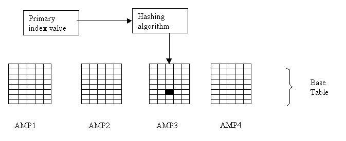
This tutorial will help you in understanding Primary Index in a much clearer way. As we saw last time a Primary Index determines the distribution of the rows  on the disks controlled AMPs. A primary index in Teradata in required for row distribution and storage. 

Below image shows how the distribution takes place using the Primary Indexes: 

The PI for a table should represent the data values used by SQL to access the data for the table. Therefore, a PI for a table should be selected very carefully as it can improve or degrade the performance of SQL used for accessing that table. 

Rules for Defining a PRIMARY INDEX

Below are some rules that I have come across while identifying on which column to be defined as PI:

* The PI selected should be such that it has unique index as more the unique index more evenly the rows will be distributed by the AMPs and better will be the space utilization.

* Define the index on as few columns as you can. 

* The PI defined can have unique or non-unique values. If defined as unique then you will have to make sure that the each value you pass into the column is unique and never repeated whereas if defined non-unique you can pass duplicate values into that column.

* Flags and Junk Dimensions are never to be defined as PI as it leads to more skewness. Therefore that data in skewed and when you perform a join it can hamper the performance and lead to spool space error.

NOTE: 

If you forget to define PRIMARY INDEX while doing a CREATE TABLE, the default will be use i.e. on the following:

* PRIMARY key

* First UNIQUE constraint

* First column

Creating PRIMARY INDEX

Unique primary index in created using the (UNIQUE) PRIMARY INDEX clause in the CREATE TABLE statement. Non-unique primary index are also created in the same way just removing the (UNIQUE) clause.

NOTE : Once a PRIMARY INDEX in created on TABLE it cannot be dropped or modified, the index must be changed by recreating the TABLE.

Example: Creating a UNIQUE PRIMARY INDEX

CREATE TABLE EMPLOYEE
(EMP_ID INTEGER
, EMP_NAME CHAR(15)
, EMP_GRADE CHAR(1))
 UNIQUE PRIMARY INDEX (EMP_ID);

Example: Creating a NON-UNIQUE PRIMARY INDEX

CREATE TABLE STUDENT
(STUDENT_ID CHAR(15)
, STUDENT_NAME CHAR(20)
, DEPARTMENT CHAR(10)) 
PRIMARY INDEX (STUDENT_ID);

Data Access using PI

When a query contains a WHERE clause, and it has primary index value(s), the request in then processed by hashing the values to find the AMP where the row is stored and then the row which contains the same hash value in the RowID part of it is returned.

Primary Key vs Primary Index

I have seen many people who are working on Teradata still confuse between Primary Key and Primary Index. So here I have done a small comparison between both as both differ conceptually:

Term	Primary Key	Primary Index
Requirement	Not required, unless referential integrity checks are to be performed	Required
Defining	Define by CREATE TABLE statement	Defined by CREATE TABLE statement
Uniqueness	Unique	Unique or non-unique
Function	Identifies a row uniquely	Distributes rows
Values can be changed?	No	Yes
Can be null?	No	Yes
Related to access path?	No	Yes

Hope this tutorial and the above short comparison helps everyone to understand what exactly PRIMARY INDEX is and how is should be chosen and defined. Do let me know your views about the post and help me in improving it.

Read More

Indexes in Teradata

Teradata as we all know is a Relational Database Management System (RDBMS) for the world's largest commercial databases. It is the market leader in  Data Warehousing. Its architecture is so designed that it takes advantage of the concept of parallelism.

Almost every Database has what we know as KEY i.e. Primary Key, Foreign Key etc defined while implementing the DDL of a table. But in Teradata we don't have any concept of Keys instead what we have is INDEX. Indexes are conceptually different from keys. PRIMARY KEY is relational modelling term that defines, in the logical model whereas the PRIMARY INDEX is a physical database implementation term that defines the actual columns used to distribute and access rows in a table.

What is an Index?

In the Teradata RDBMS, an index is used to define row uniqueness and retrieve data rows, it also can be used to enforce the primary key and unique constraint for a table. The Teradata RDBMS support five types of indexes:

* Unique Primary Index (UPI)
* Unique Secondary Index (USI)
* Non-Unique Primary Index (NUPI)
* Non-Unique Secondary Index (NUSI)
* Join Index

A typical index contains two fields:

* A Value
* A Pointer to instances of the value in a data table

Teradata uses the index and hashing to distribute rows across the AMPs, the value is condensed into an entity called a row hash.

The following rules apply to the indexes:

* As mentioned above index help in distribution and retrieval of rows of a table. It can be made up of one or more than one column.
* A table can have a number of indexes, including 1 Primary Index and more than 32 Secondary Index.
* An index defined for a table can be primary or secondary, and can be unique or non-unique. Each type of index affects the performance of the system and also the data integrity.
* An index is generally defined on columns of a table which are generally used in WHERE or join condition.
* Index helps in enforcing PRIMARY KEY and UNIQUE constraint.

Primary Index

Primary Index determines the distribution of the rows on the disks controlled AMPs. A primary index in Teradata RDBMS is required for row distribution and storage. When a row is inserted, its hash code is calculated using a hashing algorithm and depending on the whether the index is UNIQUE or Non-UNIQUE it is checked for duplication of those index. Rows having the same hash value are stored on the AMP.

Secondary Index

In addition to a primary index, up to 32 unique and non-unique secondary indexes can be defined to a table. Comparing to primary indexes, Secondary indexes allow an alternate path to access the rows in the table which is less frequently used. Basically a Secondary Index is a subtable that is stored in all AMPs separately from the primary table. The subtable made and maintained by the system contains the following information:

* RowIDs of the subtable rows
* Base table index column values
* RowIDs of the base table rows

Below diagram shows how the secondary index subtable on each AMP is associated with the base table by the RowIDs:

Join Index

A join index is nothing but an indexing structure which contains columns from multiple tables. Rather than having to join individual tables each time the join  operation is needed, the query can be resolved via a join index and in most cases dramatically improves performance.

SYNTAX:

CREATE JOIN INDEX [<database-name>.]<index_name>
[[NO] FALLBACK]
AS SELECT
[<columns>]
[SUM numeric-expression]
[COUNT coulmn-expression]
[EXTRACT year|month from date-expressino]
FROM [<database-name(s).]<table-names>]
[WHERE <search-condition>]
[GROUP BY <coulmn-name>]
[ORDER BY <coulmn-name>]
PRIMARY INDEX(<column-name>)
[index <column-name> ORDER by HASH|VALUES]
;

Read More

QuickSort Algorithm Tutorial

We have already done tutorial on Merge Sort and a tutorial on Heap Sort (Array Based) with both having a time complexity of O(n*log n). Here is another algorithm which has a time complexity of O(n*log n) and it's called QuickSort.

QuickSort as we all know has a similar approach to Merge Sort i.e. it uses Divide-and-Conquer recursive algorithm to sort the values. The difference being is it's an in-place sorting algorithm.

Basically an in-place algorithm is one which transforms the input using a data structure with a small, constant amount of extra storage space.

Read More

Binary Search Tree (BST) Algorithm Tutorial

Earlier we had a tutorial on Binary Seach Tree Basics, which you can check for refreshing the knowledge about it. Today we will be taking a look on BST algorithm and implementing it using Java.

Binary Search Tree is node based binary tree data structure with the following properties:

* The Left subtree contains the nodes with keys less than the node's key.
* The Right subtree contains the nodes with keys greater than the node's key.
* Both the right and left subtree should also be binary search tree.
* There should not be any duplicate nodes.

We have implemented below operations of Binary Search Tree:

* Searching
* Insert Node
* MinValue
* MaxValue

We will be seeing each of the operation and the corresponding Java code.

Read More

Data Warehouse Design Approaches

In our previous posts we have got to learn about Data Warehousing Objects, different kinds of Data Warehouse schemas and Data Warehouse Basics. Now it time we learn about how to build or design a Data Warehouse. 

Designing or Building of a Data Warehouse can be done following either one of the approaches. These approaches are notably known as:

* The Top-Down Approach

* The Bottom-Up Approach

These approaches are defined by the two of the bearers of Data Warehousing namely Ralph Kimball and Bill Inmon.

Read More

Data Warehousing Object: Dimension Tables Types

We had our last post on Fact Tables in Data Warehousing. This post is on Dimension Table Types. Along with Fact Tables there are many types of Dimension Tables which are used in Data Warehousing.

Dimension Tables are those tables which contain attributes that helps in describing the facts of the fact table.

The following are types of Dimension Tables:

* Slowly Changing Dimensions
* Junk Dimensions
* Confirmed Dimensions
* Degenerated Dimensions

Read More

Creating and using String Variables in visual basic

In today's tutorial I am going to be showing you how to declare and use string variables in visual basic 2010. The very basics of what you need to know about string variables are it will store a string of characters with a label name which you can then call upon later on in your programme. This can save you time as it reduces the amount of code you will have to write.

Read More

Data Warehousing Object : Fact Tables

In the previous post on DW we saw different types of Data Warehousing Schemas. So the different types of schemas had one thing in common and that was, they had Fact and Dimension Tables. So these are nothing but Data Warehousing Objects. 

Apart from Fact Tables, Dimension Tables there are other things which come under Data Warehousing Objects, they are:

* Fact Tables

* Dimension Tables

* Hierarchies

* Unique Identifiers

* Relationships

In today's post we will be taking a look in Fact tables.

Read More

I want my KAJU KATLI. Do you?

An off the topic post on Code 2 Learn, as KAJU KATLI made me go WOW!!. 

You all might be thinking why am I referring to KAJU KATLI and why am I saying "I want my KAJU KATLI". 

A friend of mine, who is an entrepreneur, a blogger and a creative genius did some research on Google's Android OS naming convention. We all at Code 2 Learn are very aware of the naming conventions in programming languages, but we never noticed that Google also follows a certain pattern to name its Android OS. 

Read More

Count the number of lines in a File in UNIX

UNIX doesn't have any real command which helps us to get the number of lines which has records or data in it. But what UNIX offers is to get the number of new lines.

The command wc -l <file_name> gives us the number of new line characters and not the no. of lines which has data. For Example, in UNIX make a file, open it and then press enter (dont write anything). Now for the same file run the above command, you will find that it returns an output as 1, which is wrong as it should return 0 as the file has no data in it.

Therefore, to overcome this shortcoming of wc -l, I thought of writing a Shell script which will give us the exact count of the number lines which has data in it.

Read More

Data Warehousing SCHEMAS

A schema is a collection of database objects, including table, views, indexes and synonyms.

There are some special architectures which arranges the schema objects in the schemas models. The most common of them are :

* Star Schema
* Snowflake Schema
* Fact constellation Schema

Read More

What is a Data Warehouse?

A very exciting and one of the hottest topic currently in the IT world is DATA WAREHOUSE. The tools which are used for the same are among some of the hot skills example INFORMATICA, TERADATA etc.

Read More

Iterative Statements in PL/SQL

In the last post on PL/SQL, we had seen Conditional Statements and how they can be used. Today we will be learning about Iterative Statements in PL/SQL.

As we all know the types of Iterative statements that are there in a programming language. PL/SQL also has the same iterative statements and the functioning is also the same, but the only thing different is their syntax. 

So lets not waste any time and move on to the topic.

Read More